Building a Deep Learning Model to Solve Sudoku: A Case Study with CNNs

Deep Learning Project

May 25, 2023 Qichun (Jackson) Yu

Abstract

Sudoku is a number puzzle game that requires you to fill in digits 1 to 9. The game requires digits 1 to 9 to appear exactly once in each row, column and each of the nine 3x3 subgrids. The project experiment with different neural networks such as CNN. The data have been divided by 9 and subtracted by 0.5 to achieve zero mean-centred data. The CNN model that includes 9 convolution layers with 512 kernels works best with 95% of training accuracy. The study found that an increase in the number of epochs, number of layers, and number of neurons per layer can help improve the accuracy of the neural network model. Moreover, the dropout layer and maxpooling can help prevent overfitting. Adding strides of 3 x 3 is useful but requires large computing power. The main objective of this project is to build a deep learning model for a mobile app company that can analyze the grid of Sudoku to be filled, solve the Sudoku problem, and fill the grid. The convolution neural networks (CNN) is good at extracting features from the dataset and can be used to solve a sudoku game successfully.

Use Case

A mobile app company is building a classical Sudoku game. The development team is working on building a deep learning model which can analyze the grid of sudoku puzzles to be filled, solve the sudoku puzzles problem, and then automatically fill the grid in the end. The dataset includes 1 million Sudoku quizzes with the solution. This deep learning model will be part of a larger code as the backend of the Sudoku game application.

Load and Read the Data

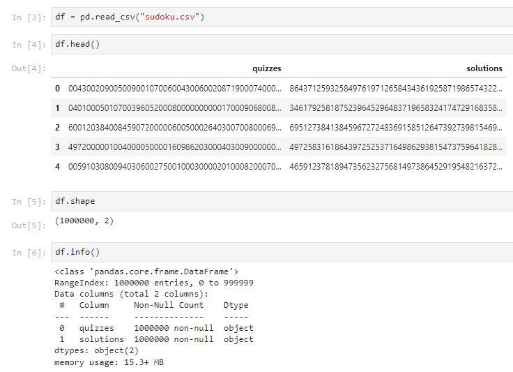
There are 1,000,000 rows with 2 columns (quizzes and solutions). The data type for each column is an object. They are both relevant to the use case and will be used to train in the model.

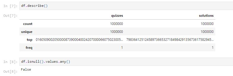
There are 1,000,000 unique quizzes and solutions. There is not null value in the dataset.

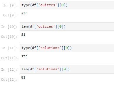
The value of the quizzes and the solutions columns are in the form of strings with a length of 81.

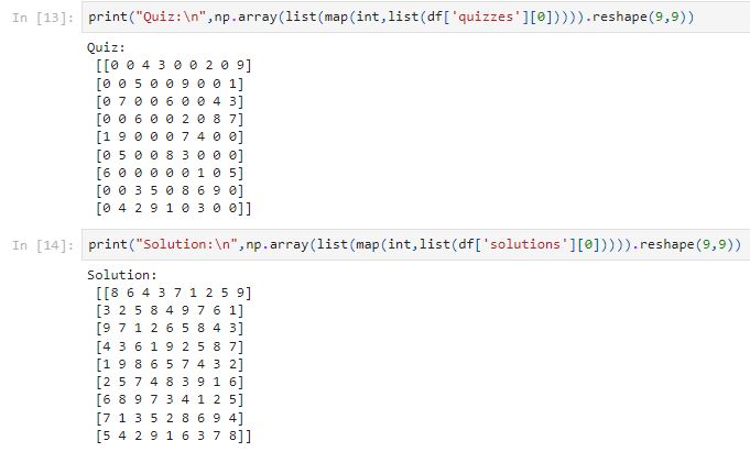
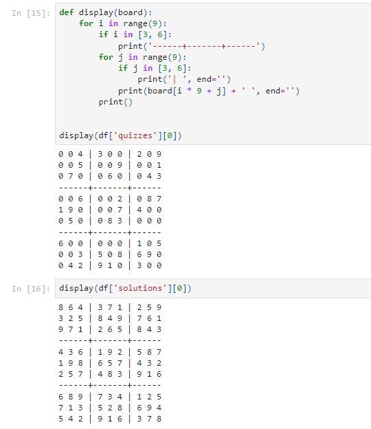
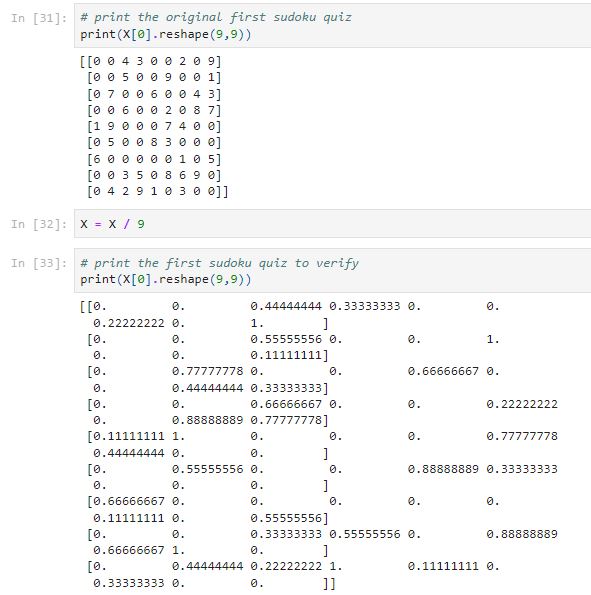
We can use reshape function to represent the puzzle as a 9X9 Python NumPy array. In the quizzes column, ‘0’ is represented as the blank. Let’s use reshape to print out the first row of the quiz and solution:

Let’s build a display function to display the puzzle board.

Let’s discover the number of blank squares in each quiz:

From the data above, we can see the number of blanks is between 44 to 52. The percentage of blanks is between 54%(47/81) to 64%(52/81). The number of given numbers is between 29 (81–52) to 37 (81–47). According to ResearchGate, the number of clues between 28–31 is considered to be difficult, the number of clues between 32–35 is considered to be medium difficulty level, and the number of clues between 36–46 is considered to be easy. Therefore, most of the Sudoku quizzes from this dataset are considered to be medium. (https://www.researchgate.net/figure/Number-of-clues-for-each-difficulty-level_tbl1_259525699)

sns.countplot(x=df['number_of_blanks'])

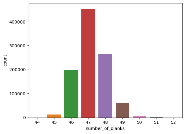
From the plot above, most of the puzzle has 47 blank grids.

fig1, ax1 = plt.subplots(figsize=(8, 8))
ax1.pie(df['number_of_blanks'].value_counts(), autopct='%1.2f%%', pctdistance=1.1)
ax1.legend(df['number_of_blanks'].value_counts().index)
ax1.axis('equal')  # Equal aspect ratio ensures that pie is drawn as a circle.

plt.title("Percentage by the Number of Blanks Cells in the quizzes")
plt.show()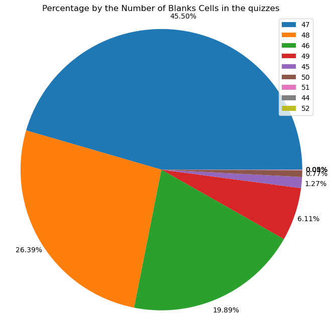

From the pie chart above, we can see about 45.5% of quizzes with 47 blank cells. The medium difficulty level (46–49 blanks) is about 98% (45.50%+26.39%+19.89%+6.11%).

Before the model building, it is important to verify that all the solutions are valid sudoku solutions. A solution is valid must be validated with the following rules:

Each row must contain 1–9 without repetition
Each column must contain 1–9 without repetition
Each of the nine 3 x 3 sub-squares must contain 1–9 without repetition

Preprocessing

Before passing the data as inputs to the neural net model, use reshape function from NumPy to expand the dimensions (N, 9, 9, -1).

X = np.array(df.quizzes.map(lambda x: list(map(int, x))).to_list()).reshape(-1,9,9,1)
Y = np.array(df.solutions.map(lambda x: list(map(int, x))).to_list()).reshape(-1,9,9)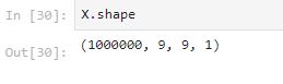

Normalization

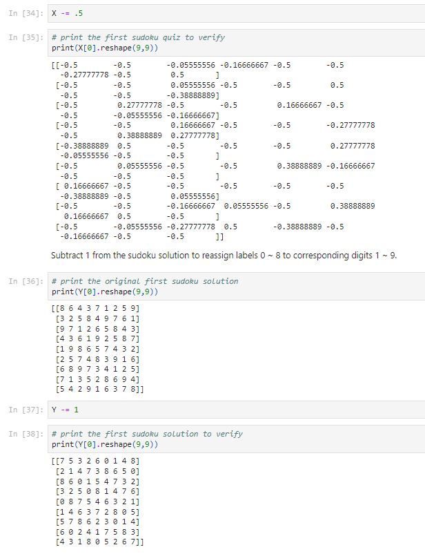
Normalize the data by dividing it by 9 and subtracting it by 0.5 to achieve zero mean-centred data. Because the neural networks usually generate a better performance with zero-centred normalized data.

Data Splitting

Splitting data with a ratio of 80/20. The first 800,000 data (80%) as the training set and the last 200,000 data (20%) as the testing set.

# set training split equal to 0.8
training_split = 0.8

splitidx = int(len(data) * training_split)
# first 80% of data as training set, last 20% of data as testing set
x_train, x_test = X[:splitidx], X[splitidx:]
y_train, y_test = Y[:splitidx], Y[splitidx:]

Neural Networks Models

Visualizing the Loss & Accuracy Plot of Training & Validation data can help us to know if a model has overfitting or underfitting. Matplotlib plots can help us visualize the history of network learning (accuracy & loss).

If loss falls on the training set and increases on the testing set, the network model has overfitted.
Training loss is much lower than validation loss, the network is overfitting.
If the training loss is too high, it indicates the neural network model could not learn the training data and the network is underfitting.

# define a plot function to plot the loss and accuracy of train and test
def loss_acc_plot(history):
	fig, ax = plt.subplots(1,2)
	fig.set_size_inches(12,6)

	ax[0].plot(history.history['loss'], label='train loss')
	ax[0].plot(history.history['val_loss'], label='val loss')
	ax[0].set_title('Training and Validation Loss')
	ax[0].set_ylabel('Loss')
	ax[0].set_xlabel('Epochs')
	ax[0].legend(['train', 'val'], loc='upper right')

	ax[1].plot(history.history['accuracy'], label='accuracy')
	ax[1].plot(history.history['val_accuracy'], label='val_accuracy')
	ax[1].set_title('Training and Validation Accuracy')
	ax[1].set_ylabel('Accuracy')
	ax[1].set_xlabel('Epochs')
	ax[1].legend(['train', 'val'], loc='upper right')

	plt.show()

The models use Adam Optimizer with a learning rate of 0.001, the optimizer is save to a variable called optimizer.

# using an Adam optimizer with a learning rate of 0.001
optimizer = tf.keras.optimizers.Adam(0.001)

Because we are training a multiclass classifier, predicting digits 1~9 (9 classes). Since we are not using one-hot encoded, the loss function that is using is sparse_categorical_crossentropy. For multi-class classification, Softmax will be the activation function for the last layer, which outputs multiple numerical numbers ranging from 0 to 8 (9 classes)corresponding to the probability of each class.

Convolutional Neural Networks (CNNs)

Convolutional neural networks (CNN) are good at extracting local features from the image and are commonly used to analyze visual imagery. If we treat each number as its own feature of the puzzle, so there are 81 different features available. CNN is good at extracting features, which could generate good performance.

Hyperparameter Tuning:

Number of epochs: Increasing the number of epochs can help improve the accuracy and lowers the loss; however, a high number of epochs may result in an overfitting model.
Number of layers: Increasing the number of layers help increases the accuracy; however, a high number of layers may result in an overfitting model.
Number of neurons per layer: Increasing the number of neurons can help improve the accuracy.

CNN Model 1

Let’s start with a simple CNN model.

The model starts with a Conv2D() class, which is a 2D convolution layer. The first layer is a convolution layer with 64 kernels that are (3,3) in dimension. The padding is ‘same’ so that the padding gets the same output dimension as the input. The ReLU is used as the activation function. The input is batches of arrays of shape (9,9).
Batch normalization is a method to normalize the inputs of each layer. It can help speed up and stabilize neural networks.
Adding a convolution layer with 64 kernels of shape (3 x 3), a batch normalization layer and a convolution layer with 128 kernels of shape (1 x 1).
After that, a Flatten layer helps to comprise the (9,9, 128) to 10,368 (9x9x128) input nodes.
Dense is a regular neural network layer that performs a dot product operation. The matrix multiplication is represented by the dot(X, W) + B, where X is the input to the layer, W is the weight, and B is the bias. Using 729 (81x9) in the dense layer means performing matrix multiplication to result in an output matrix with a desired last dimension to be 729.
LayerNormalization is used to normalize a layer.
Using Reshape layer to (9,9,9) so that the last layer has 9 neurons corresponding to the 9 classes(0~8) with a softmax activation function.

# Function for the cnn model function
def cnn_model_func1():
	# Instantiate model
	model = tf.keras.Sequential()
	# add a convolution layer with 64 kernels of shape (3 x 3)
	model.add(Conv2D(64, kernel_size=(3,3), activation='relu', padding='same', input_shape=(9,9,1)))
	# normalize the kernel values for Convolution Layers
	model.add(BatchNormalization())
	# add a convolution layer with 64 kernels of shape (3 x 3)
	model.add(Conv2D(64, kernel_size=(3,3), activation='relu', padding='same'))
	# normalize the kernel values for Convolution Layers
	model.add(BatchNormalization())
	# add a convolution layer with 128 kernels of shape (1 x 1)
	model.add(Conv2D(128, kernel_size=(1,1), activation='relu', padding='same'))
	# comprises the (9,9, 128) to a 10,368 (9*9*128) input nodes
	model.add(Flatten())
	# Add a dense layer to perform matrix multiplication to result in an output matix with 729(81*9)
	model.add(Dense(81*9))
	# normalize the dense layer above
	model.add(LayerNormalization(axis=-1))
	# the last layer has 9 neurons corresponding to the 9 classes with a softmax activation function
	model.add(Reshape((9, 9, 9)))
	# using softmax as activation function for multiclass
	model.add(Activation('softmax'))

	return model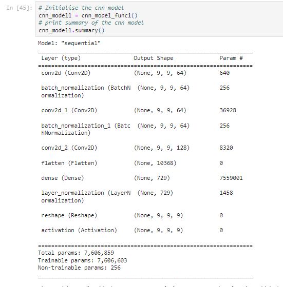

The model compiles with the sparse_categorical_crossentropy loss function which does not require passing one-hot vectors as output. Training with a batch size of 32 and epochs of 5. Batch size is the number of samples processed before the network model is updated. Large batch size may result in overfitting so the model starts with 32. Let’s train it with five epochs to see how it performs.

									# Train the model
cnn_model1.compile(loss='sparse_categorical_crossentropy', optimizer=optimizer, metrics=['accuracy'])

history1 = cnn_model1.fit(x_train, y_train, batch_size=32, epochs=5, validation_data=(x_test, y_test))

loss_acc_plot(history1)

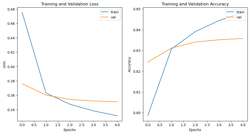
From the above training, it looks like the training loss decreasing but the validation loss is increasing. The model is overfitting.

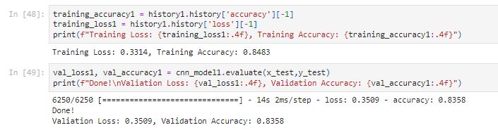
The training accuracy of 0.8483 is not bad. But let’s test the model to see if it can solve a real sudoku game or not.

From above, we can see the model is making some bad predictions with the first training quiz.

CNN Model 1 only achieved an accuracy of 84% on the training set and is not ideal for solving a sudoku game since it is making bad predictions on the real sudoku game. Let’s see if we can create a better model for solving the sudoku game.

CNN Model 2

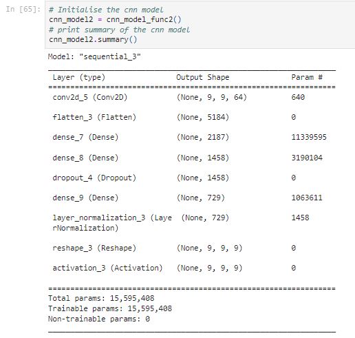
Let’s try another simple CNN model.

The model starts with a Conv2D() class, which is a 2D convolution layer. The first layer is a convolution layer with 64 kernels that are (3,3) in dimension. The padding is ‘same’ so that a padding gets the same output dimension as the input. The ReLU is used as the activation function.
After that, a Flatten layer helps to comprise the (9,9, 64) to 5,184 (9x9x64) input nodes.
Add a Dense layer that performs a dot product operation. Using 2187 (81x9x3) in the dense layer means performing matrix multiplication to result in an output matrix with a desired last dimension to be 2187.
Add a Dense layer that performs a dot product operation. Using 1458 (81x9x2) in the dense layer means performing matrix multiplication to result in an output matrix with a desired last dimension to be 1458.
A Dropout of 20% is added to the hidden layer. A dropout method randomly deactivated a certain number of neurons during the training process. Adding a dropout of 20% means 20% of the neurons in that layer will be randomly deactivated during training.
Add a Dense layer that performs a dot product operation. Using 729 (81x9) in the dense layer means performing matrix multiplication to result in an output matrix with a desired last dimension to be 729.
LayerNormalization is used to normalize a layer.
Using Reshape layer to (9,9,9) so that the last layer has 9 neurons corresponding to the 9 classes(0~8) with a softmax activation function.

									def cnn_model_func2():
	# Instantiate model
	model = tf.keras.Sequential()
	# add a convolutiion layer with 64 kernels of shape (3 x 3)
	model.add(Conv2D(64, kernel_size=(3,3), activation='relu', padding='same', input_shape=(9,9,1)))
	# comprise the (9 , 9 , 64) to 5184 input nodes
	model.add(Flatten())
	# add a dense layer (81 * 9 *3)
	model.add(Dense(81*9*3, activation='relu'))
	 # add a dense layer (81 * 9 *2)
	model.add(Dense(81*9*2, activation='relu'))
	# add a dropout layer of 20% to prevent overfitting
	model.add(Dropout(.20))
	 # add a dense layer (81 * 9 )
	model.add(Dense(81*9, activation='relu'))
	# normalize the dense layer 
	model.add(LayerNormalization(axis=-1))
	# reshape and using softmax as activation function for multiclass
	model.add(Reshape((9, 9, 9)))
	model.add(Activation('softmax'))

	return model

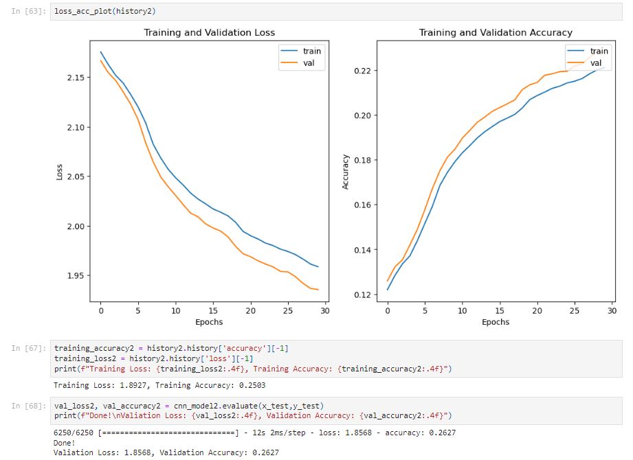
After 100 epochs, the training accuracy is only 0.2503. The model takes a longer time to train and the prediction is low. The model is underfitting.

CNN Model 3

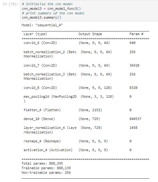
Let’s build on top of the CNN Model 1 with MaxPooling.

Pooling layers can help to reduce the dimensions of the feature maps of convolution. It can help the model focus only on the detected pattern. Max Pooling will find the maximum values at a specific area of the feature map. Adding pooling layers can help speed up the training time and reduce overfitting issues.

The model is using MaxPooling2d with (3,3) since it makes sense with a 9 X 9 sudoku board game.

									def cnn_model_func3():

	model = tf.keras.Sequential()
	model.add(Conv2D(64, kernel_size=(3,3), activation='relu', padding='same', input_shape=(9,9,1)))
	model.add(BatchNormalization())
	model.add(Conv2D(64, kernel_size=(3,3), activation='relu', padding='same'))
	model.add(BatchNormalization())
	model.add(Conv2D(128, kernel_size=(1,1), activation='relu', padding='same'))

	# adding MaxPooling layer
	model.add(MaxPooling2D(3,3))

	model.add(Flatten())
	model.add(Dense(81*9))
	model.add(tf.keras.layers.LayerNormalization(axis=-1))
	model.add(Reshape((9, 9, 9)))
	model.add(Activation('softmax'))

	return model

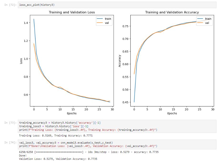
After 30 epochs, the model has a training accuracy of 0.7771. The training accuracy is still low.

CNN Model 4

Let’s build on top of the CNN Model 1 with strides of (3x3). Considering a valid Sudoku solution must follow each of the nine 3 X 3 sub-squares must contain 1–9 without repetition.

Stride defines how many steps we are moving in each step in convolution. Using a stride of (3,3) means the convolution moving each of the nine 3 x 3 sub-squares.

Since the first model was overfitting. Let’s add a Dropout layer of 20%.

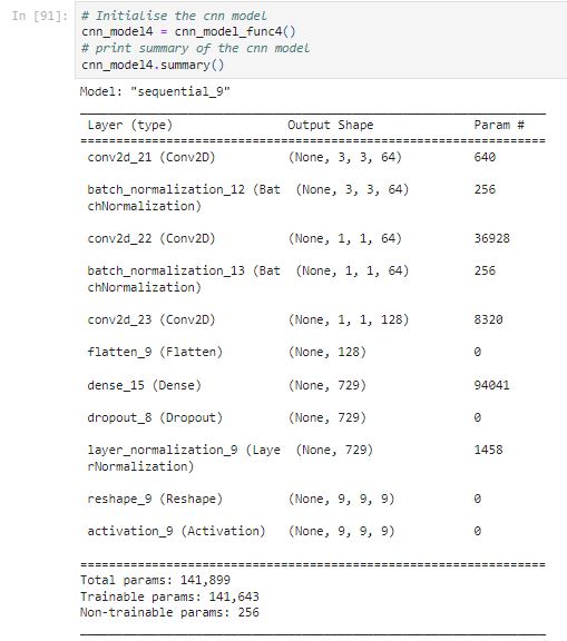
# Function for the cnn model function def cnn_model_func4(): model = tf.keras.Sequential() # add a convolution layer with 64 kernels of shape (3 x 3), strides (3,3) model.add(Conv2D(64, kernel_size=(3,3), strides=(3,3), activation='relu', padding='same', input_shape=(9,9,1))) model.add(BatchNormalization()) model.add(Conv2D(64, kernel_size=(3,3), strides=(3,3), activation='relu', padding='same')) model.add(BatchNormalization()) model.add(Conv2D(128, kernel_size=(1,1), strides=(3,3), activation='relu', padding='same')) model.add(Flatten()) model.add(Dense(81*9)) # add a dropout layer of 10% to prevent overfitting model.add(Dropout(.10)) model.add(tf.keras.layers.LayerNormalization(axis=-1)) model.add(Reshape((9, 9, 9))) model.add(Activation('softmax')) return model

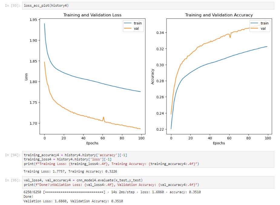
After 100 epochs, the model generates a training accuracy of 0.3326. The model takes a longer time to train and the model is underfitting. After adding the dropout, the validation accuracy is higher than the training accuracy because adding a 20% dropout means 20% of the features are set to zero. When validating, all features are used so it can lead to higher validation accuracy.

CNN Model 5

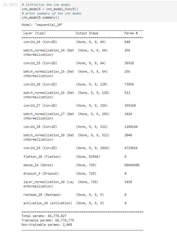
Let’s add more layers and increase the number of neurons to see if the model performs better.

# Function for the cnn model function def cnn_model_func5(): model = tf.keras.Sequential() model.add(Conv2D(64, kernel_size=(3,3), activation='relu', padding='same', input_shape=(9,9,1))) model.add(BatchNormalization()) model.add(Conv2D(64, kernel_size=(3,3), activation='relu', padding='same')) model.add(BatchNormalization()) model.add(Conv2D(128, kernel_size=(3,3), activation='relu', padding='same')) model.add(BatchNormalization()) model.add(Conv2D(256, kernel_size=(3,3), activation='relu', padding='same')) model.add(BatchNormalization()) model.add(Conv2D(512, kernel_size=(3,3), activation='relu', padding='same')) model.add(BatchNormalization()) model.add(Conv2D(1024, kernel_size=(3,3), activation='relu', padding='same')) model.add(Flatten()) model.add(Dense(81*9)) # add a dropout layer of 10% to prevent overfitting model.add(Dropout(.1)) model.add(tf.keras.layers.LayerNormalization(axis=-1)) model.add(Reshape((9, 9, 9))) model.add(Activation('softmax')) return model

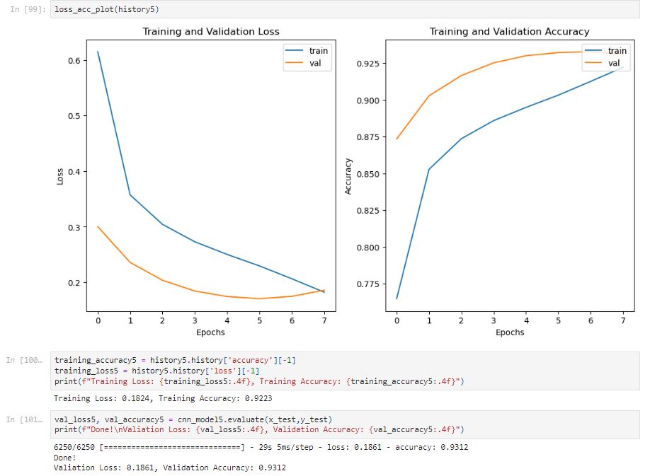
After 8 epochs, the training accuracy is 0.9223 and the validation accuracy is 0.9312. This is a high accuracy; however, if we check the graph that compared the training and validation loss, we can see that the model is overfitting after five epochs since the validation loss is increasing but the training loss is still decreasing.

CNN Model 6

Adding strides of (3x3) to see how it performs.

# Function for the cnn model function def cnn_model_func6(): model = tf.keras.Sequential() model.add(Conv2D(32, kernel_size=(3,3), strides=(3,3), activation='relu', padding='same', input_shape=(9,9,1))) model.add(BatchNormalization()) model.add(Conv2D(64, kernel_size=(3,3), strides=(3,3), activation='relu', padding='same')) model.add(BatchNormalization()) model.add(Conv2D(128, kernel_size=(3,3), strides=(3,3), activation='relu', padding='same')) model.add(BatchNormalization()) model.add(Conv2D(256, kernel_size=(3,3), strides=(3,3), activation='relu', padding='same')) model.add(BatchNormalization()) model.add(Conv2D(512, kernel_size=(3,3), strides=(3,3), activation='relu', padding='same')) model.add(BatchNormalization()) model.add(Conv2D(1024, kernel_size=(3,3), strides=(3,3), activation='relu', padding='same')) model.add(Flatten()) model.add(Dense(512,activation='relu')) model.add(Dropout(0.1)) model.add(Dense(81*9)) model.add(tf.keras.layers.LayerNormalization(axis=-1)) model.add(Reshape((9, 9, 9))) model.add(Activation('softmax')) return model

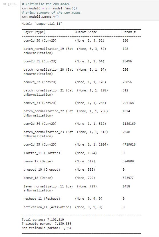
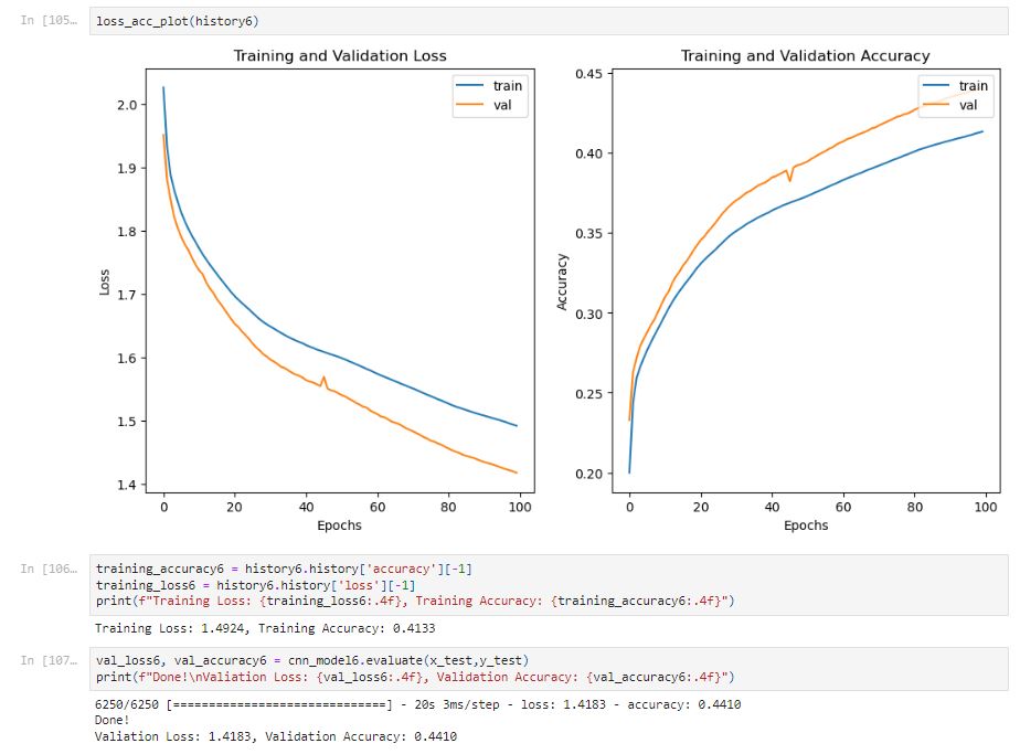
After 100 epochs, the training accuracy is only 41.33%. The model is underfitting.

CNN Model 7

Testing model with strides of (2x2).

def cnn_model_func7(): model = tf.keras.Sequential() model.add(Conv2D(32, kernel_size=(3,3), strides=(2,2), activation='relu', padding='same', input_shape=(9,9,1))) model.add(BatchNormalization()) model.add(Conv2D(64, kernel_size=(3,3), strides=(2,2), activation='relu', padding='same')) model.add(BatchNormalization()) model.add(Conv2D(128, kernel_size=(3,3), strides=(2,2), activation='relu', padding='same')) model.add(BatchNormalization()) model.add(Conv2D(256, kernel_size=(3,3), strides=(2,2), activation='relu', padding='same')) model.add(BatchNormalization()) model.add(Conv2D(512, kernel_size=(3,3), strides=(2,2), activation='relu', padding='same')) model.add(BatchNormalization()) model.add(Conv2D(1024, kernel_size=(3,3), strides=(2,2), activation='relu', padding='same')) model.add(Flatten()) model.add(Dense(512,activation='relu')) model.add(Dropout(0.1)) model.add(Dense(81*9)) model.add(tf.keras.layers.LayerNormalization(axis=-1)) model.add(Reshape((9, 9, 9))) model.add(Activation('softmax')) return model

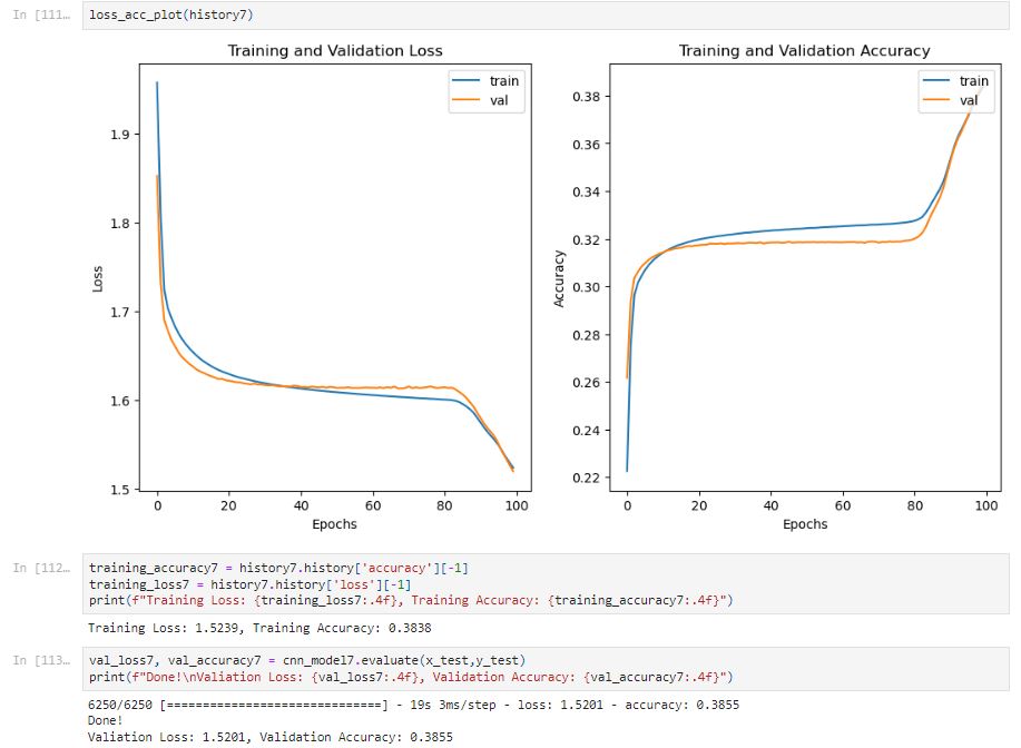
The training accuracy is 0.3838, using strides (2X2) is not preferable.

CNN Model 8

Using 6 convolution layers with 512 kernels to see if the model performance has improved.

# Function for the cnn model function def cnn_model_func8(): model = tf.keras.Sequential() model.add(Conv2D(512, kernel_size=(3,3), activation='relu', padding='same', input_shape=(9,9,1))) model.add(BatchNormalization()) model.add(Conv2D(512, kernel_size=(3,3), activation='relu', padding='same')) model.add(BatchNormalization()) model.add(Conv2D(512, kernel_size=(3,3), activation='relu', padding='same')) model.add(BatchNormalization()) model.add(Conv2D(512, kernel_size=(3,3), activation='relu', padding='same')) model.add(BatchNormalization()) model.add(Conv2D(512, kernel_size=(3,3), activation='relu', padding='same')) model.add(BatchNormalization()) model.add(Conv2D(512, kernel_size=(3,3), activation='relu', padding='same')) model.add(Flatten()) model.add(Dense(81*9)) model.add(Dropout(0.1)) model.add(tf.keras.layers.LayerNormalization(axis=-1)) model.add(Reshape((9, 9, 9))) model.add(Activation('softmax')) return model

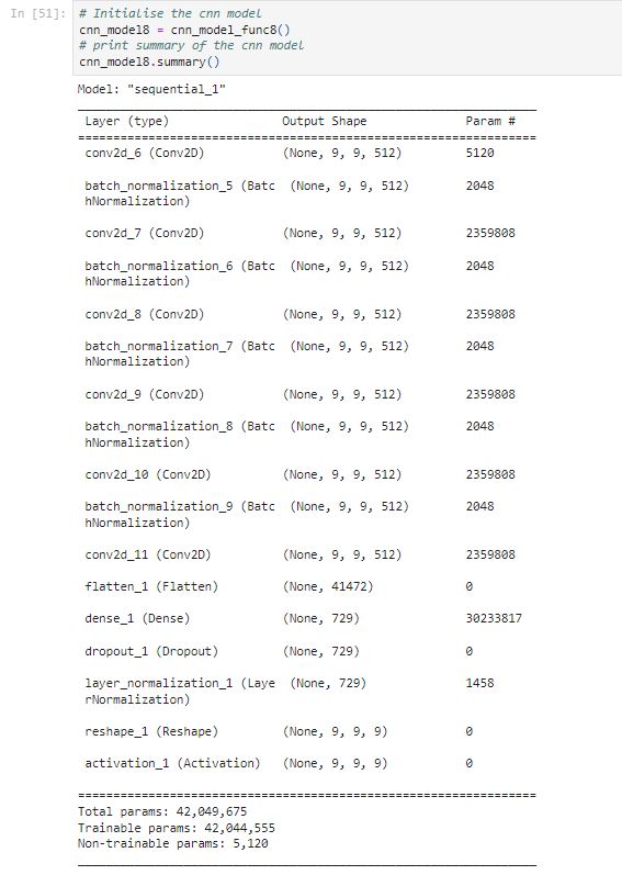
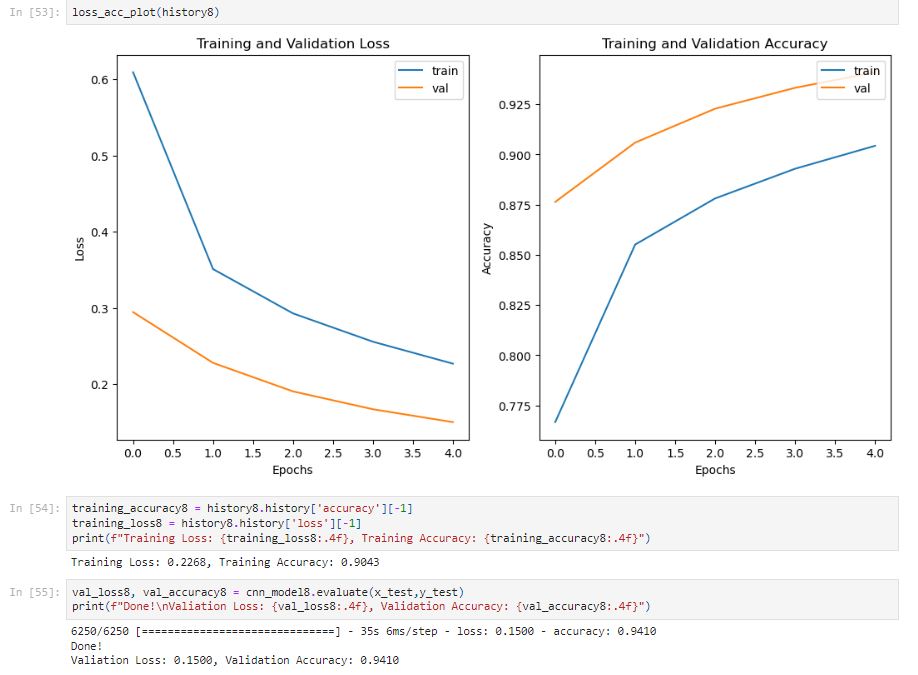
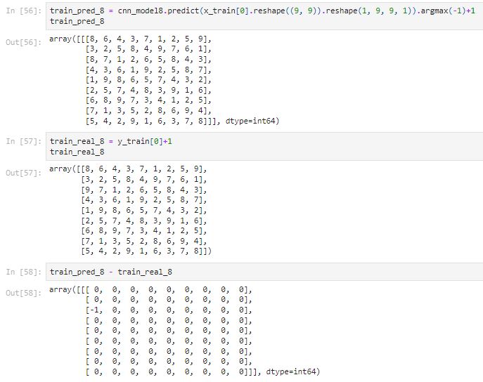
The training accuracy improved to 90.43%. From the graph above, the model doesn’t seem to be overfitting. Let’s use the model to predict the quiz to see how it performs.

CNN Model 9

Let’s build on top of the CNN Model 8 with strides of (3x3).

# Function for the cnn model function def cnn_model_func9(): model = tf.keras.Sequential() model.add(Conv2D(512, kernel_size=(3,3), strides=(3,3), activation='relu', padding='same', input_shape=(9,9,1))) model.add(BatchNormalization()) model.add(Conv2D(512, kernel_size=(3,3), strides=(3,3), activation='relu', padding='same')) model.add(BatchNormalization()) model.add(Conv2D(512, kernel_size=(3,3), strides=(3,3), activation='relu', padding='same')) model.add(BatchNormalization()) model.add(Conv2D(512, kernel_size=(3,3), strides=(3,3), activation='relu', padding='same')) model.add(BatchNormalization()) model.add(Conv2D(512, kernel_size=(3,3), strides=(3,3), activation='relu', padding='same')) model.add(BatchNormalization()) model.add(Conv2D(512, kernel_size=(3,3), strides=(3,3), activation='relu', padding='same')) model.add(Flatten()) model.add(Dense(81*9)) model.add(Dropout(0.1)) model.add(tf.keras.layers.LayerNormalization(axis=-1)) model.add(Reshape((9, 9, 9))) model.add(Activation('softmax')) return model

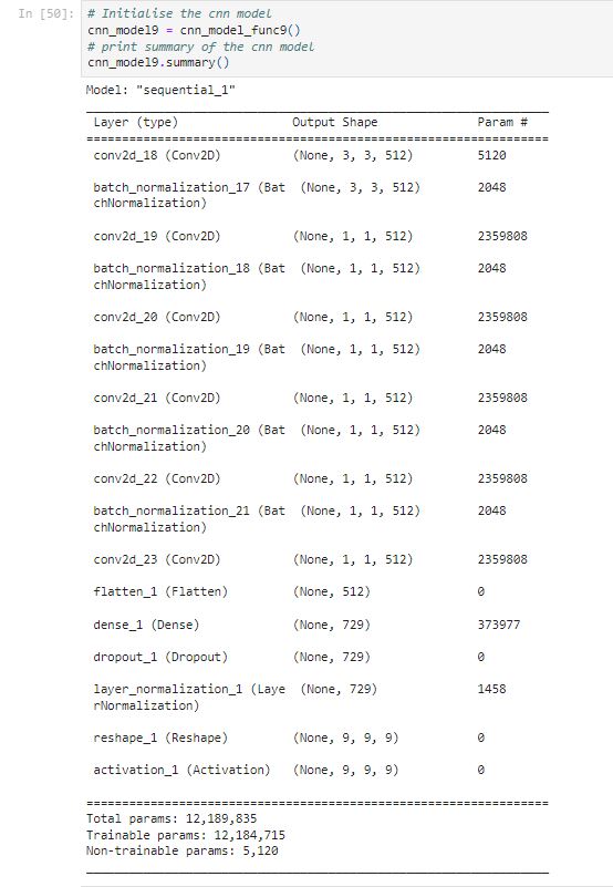
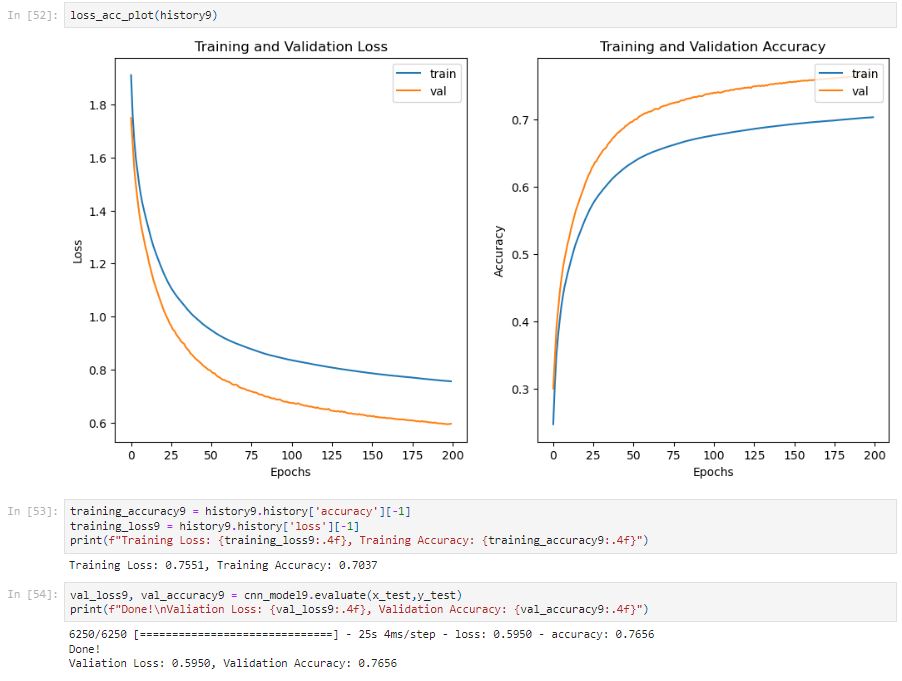
After 200 epochs, the training accuracy is only 70.37%. From the training above, we can see the accuracy is slowly increasing by 0.0002 for each epoch.

CNN Model 10

Trying with 18 conv2D layers to see if it has a better performance.

# Function for the cnn model function def cnn_model_func10(): model = tf.keras.Sequential() model.add(Conv2D(512, kernel_size=(3,3), strides=(3,3), activation='relu', padding='same', input_shape=(9,9,1))) model.add(BatchNormalization()) model.add(Conv2D(512, kernel_size=(3,3), strides=(3,3), activation='relu', padding='same')) model.add(BatchNormalization()) model.add(Conv2D(512, kernel_size=(3,3), strides=(3,3), activation='relu', padding='same')) model.add(BatchNormalization()) model.add(Conv2D(512, kernel_size=(3,3), strides=(3,3), activation='relu', padding='same')) model.add(BatchNormalization()) model.add(Conv2D(512, kernel_size=(3,3), strides=(3,3), activation='relu', padding='same')) model.add(BatchNormalization()) model.add(Conv2D(512, kernel_size=(3,3), strides=(3,3), activation='relu', padding='same')) model.add(BatchNormalization()) model.add(Conv2D(512, kernel_size=(3,3), strides=(3,3), activation='relu', padding='same')) model.add(BatchNormalization()) model.add(Conv2D(512, kernel_size=(3,3), strides=(3,3), activation='relu', padding='same')) model.add(BatchNormalization()) model.add(Conv2D(512, kernel_size=(3,3), strides=(3,3), activation='relu', padding='same')) model.add(BatchNormalization()) model.add(Conv2D(512, kernel_size=(3,3), strides=(3,3), activation='relu', padding='same')) model.add(BatchNormalization()) model.add(Conv2D(512, kernel_size=(3,3), strides=(3,3), activation='relu', padding='same')) model.add(BatchNormalization()) model.add(Conv2D(512, kernel_size=(3,3), strides=(3,3), activation='relu', padding='same')) model.add(BatchNormalization()) model.add(Conv2D(512, kernel_size=(3,3), strides=(3,3), activation='relu', padding='same')) model.add(BatchNormalization()) model.add(Conv2D(512, kernel_size=(3,3), strides=(3,3), activation='relu', padding='same')) model.add(BatchNormalization()) model.add(Conv2D(512, kernel_size=(3,3), strides=(3,3), activation='relu', padding='same')) model.add(BatchNormalization()) model.add(Conv2D(512, kernel_size=(3,3), strides=(3,3), activation='relu', padding='same')) model.add(BatchNormalization()) model.add(Conv2D(512, kernel_size=(3,3), strides=(3,3), activation='relu', padding='same')) model.add(BatchNormalization()) model.add(Conv2D(512, kernel_size=(3,3), strides=(3,3), activation='relu', padding='same')) model.add(Flatten()) model.add(Dense(81*9)) model.add(Dropout(0.2)) model.add(tf.keras.layers.LayerNormalization(axis=-1)) model.add(Reshape((9, 9, 9))) model.add(Activation('softmax')) return model

After 63 epochs with about 6 hours of training, I interrupt the training with the keyboard. The training accuracy is only 19% with a slow increase. The training is incomplete.

CNN Model 11

Testing with 9 conv2D layers, 9 is matching 9 numbers of Sudoku and the game board is 9 x 9.

# Function for the cnn model function def cnn_model_func11(): model = tf.keras.Sequential() model.add(Conv2D(512, kernel_size=(3,3), activation='relu', padding='same', input_shape=(9,9,1))) model.add(BatchNormalization()) model.add(Conv2D(512, kernel_size=(3,3), activation='relu', padding='same')) model.add(BatchNormalization()) model.add(Conv2D(512, kernel_size=(3,3), activation='relu', padding='same')) model.add(BatchNormalization()) model.add(Conv2D(512, kernel_size=(3,3), activation='relu', padding='same')) model.add(BatchNormalization()) model.add(Conv2D(512, kernel_size=(3,3), activation='relu', padding='same')) model.add(BatchNormalization()) model.add(Conv2D(512, kernel_size=(3,3), activation='relu', padding='same')) model.add(BatchNormalization()) model.add(Conv2D(512, kernel_size=(3,3), activation='relu', padding='same')) model.add(BatchNormalization()) model.add(Conv2D(512, kernel_size=(3,3), activation='relu', padding='same')) model.add(BatchNormalization()) model.add(Conv2D(512, kernel_size=(3,3), activation='relu', padding='same')) model.add(Flatten()) model.add(Dense(81*9)) model.add(Dropout(0.1)) model.add(tf.keras.layers.LayerNormalization(axis=-1)) model.add(Reshape((9, 9, 9))) model.add(Activation('softmax')) return model

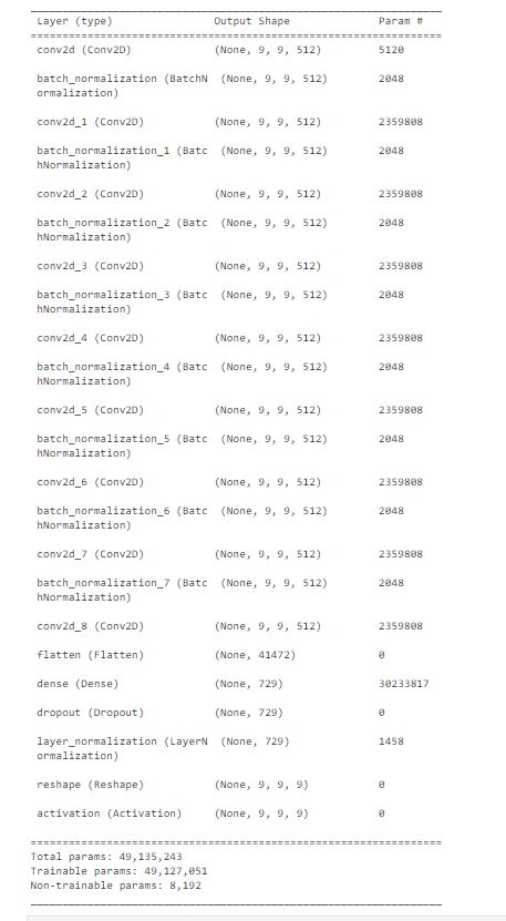
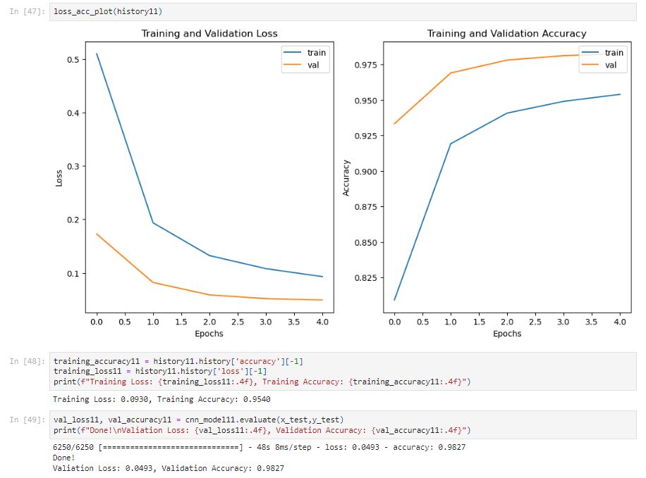
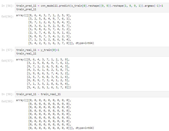
After only five epochs, the model has a 95.4% training accuracy. The model performance is desirable.

Discussion

Let’s create a summary table with for each model.

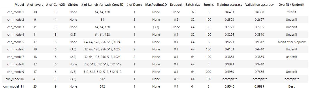
The convolution neural networks (CNN) is good at extracting features. An increase in the number of epochs, number of layers, and number of neurons per layer can help improve the accuracy of the model. In this project, we start with a simple CNN model with 3 conv2D layers. The model is overfitting. So we have tried adding a dropout layer or using maxpooling to prevent overfitting. Adding strides of (3x3) could be good considering valid sudoku must follow each of the nine 3X3 sub-squares and should contain 1–9 digits without repetition. However, models that have strides require longer training hours with more epochs.

After testing all of the models, the cnn_model_11 has the best performance in solving sudoku games with a training accuracy of 0.9540 and validation accuracy of 0.9827.

Let’s test the model to see whether it can solve a real sudoku game or not.

Confusion Matrix

Use the model to make predict all the testing data.

y_pred_11 = cnn_model11.predict(x_test)

Since we used normalization to transform the dataset before, we need to create functions to transform the prediction and the testing data back to the real board game with a dimension of (200000, 2).

def y_pred_func(len, model): list = [] for i in range(len): test_pred = model.predict(x_test[i].reshape((9, 9)).reshape(1, 9, 9, 1)).argmax(-1)+1 list.append((i, test_pred)) return np.array(list)

y_pred_11 = y_pred_func(x_test.shape[0], cnn_model11)

def y_real_func(data): len = data.shape[0] list = [] for i in range(len): y_real = data[i] +1 list.append((i, y_real)) return np.array(list) y_real_11 = y_real_func(y_test)

Create a function to calculate the accuracy for each position.

def count_grid_acc(actual, predicted): result = np.zeros((9,9), dtype=np.int) for i in range(y_real_11.shape[0]): for j in range(9): for k in range(9): if actual[i][1][j][k] == predicted[i][1][0][j][k]: result[j][k] += 1 return result

cga = count_grid_acc(y_real_11, y_pred_11)

ticks = [1,2,3,4,5,6,7,8,9] plt.figure(figsize=(20,15)) sns.heatmap(cga, annot=True, fmt='g',xticklabels = ticks, yticklabels = ticks) plt.title('Number of correct prediction for each position') plt.xlabel('Predicted') plt.ylabel('Actual')

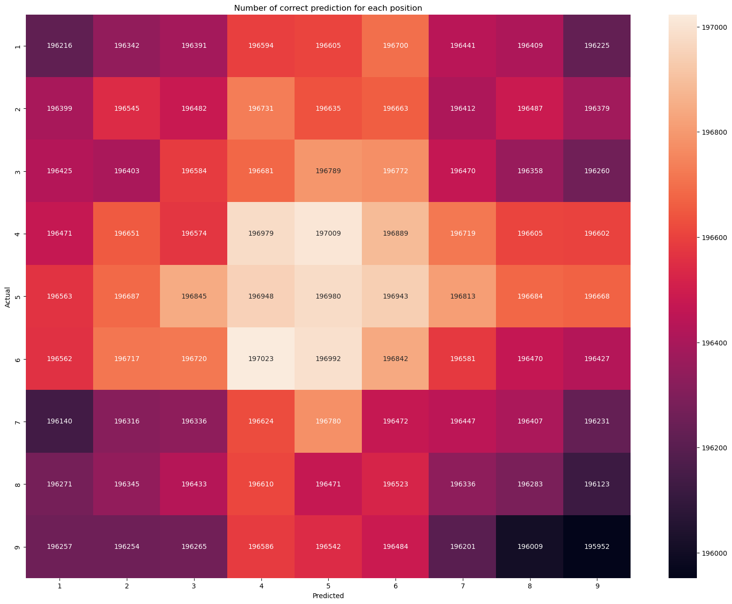
It looks like for each position, the model makes the correct prediction of about 196,500 out of 200,000. It looks pretty high, let’s build a function to check the accuracy for each position.

def count_grid_position_acc(cga): sum = y_test.shape[0] acc = np.zeros((9,9)) for i in range(9): for j in range(9): acc[i][j] = round(cga[i][j] / sum, 4) return acc cga_acc = count_grid_position_acc(cga)

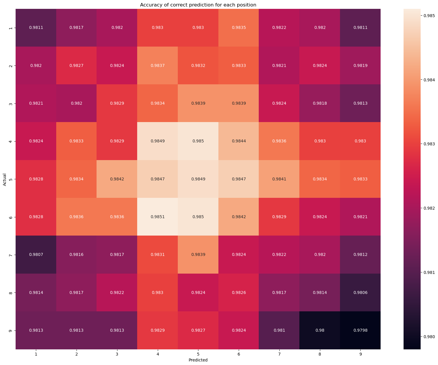
Looks like all positions are around 98% correct.

Let’s build a confusion matrix function to evaluate the model. The confusion matrix is a summary of prediction results for a classification problem. We want to evaluate to check if the model can classify the digit 1 to 9 correctly.

def confusion_matrix_func(actual, predicted): result = np.zeros((9,9), dtype=np.int) for i in range(y_real_11.shape[0]): for j in range(9): for k in range(9): if predicted[i][1][0][j][k] == actual[i][1][j][k]: result[actual[i][1][j][k]-1][actual[i][1][j][k]-1] += 1 else: result[actual[i][1][j][k]-1][predicted[i][1][0][j][k]-1] += 1 return result cm = confusion_matrix_func(y_real_11, y_pred_11)

The y-axis is the actual label and the x-axis is the predicted label. For example, the first number 1,767,456 indicates that the model predicts the number is 1 when it is actually one. This is also called a true positive. However, the second of the first row indicates the model predicts 4197 times that the digit is 2 but it is actually 1. This is also called False Negative. The first number of the second row indicates the model predicts 3863 times that the digit is 1 but it is actually 2.

Let’s build a function to calculate the accuracy for each digit.

norm_cm = np.round(cm/cm.astype(np.float).sum(axis=1), 4)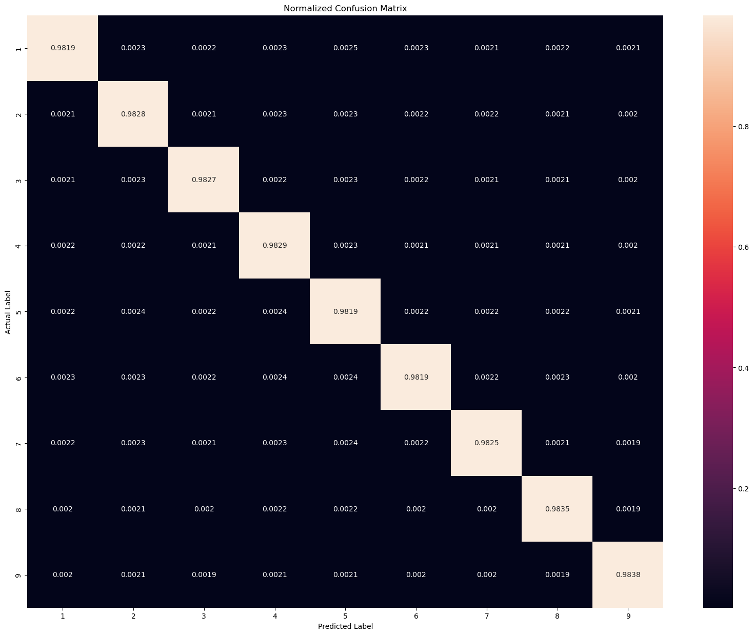

We can see there are around 98% of times the model predicts the digit is 1 when it is actually 1.

df = pd.DataFrame(cm, index= ['1','2','3','4','5','6','7','8','9'], columns=['1','2','3','4','5','6','7','8','9'], dtype=int) df.da.export_metrics()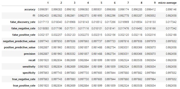

From the report above, we can see the average f1 score is 98% for this model. The F1 score encodes precision and recall. The score is high indicating the model is well performed.

Conclusion

In this study, we have experimented with different neural networks such as CNN. The above study has shown the possibility of solving sudoku games using Deep learning methods. The neural networks have better performance with zero-centred normalized data. The data have been divided by 9 and subtracted by 0.5 to achieve zero mean-centred data. The convolution neural networks (CNN) is good at extracting features. An increase in the number of epochs, number of layers, and number of neurons per layer can help improve the accuracy of the model. Dropout layer or maxpooling can help prevent overfitting. Adding strides of 3 x 3 could be useful but require large training hours and computing power.

From the above experiments with different neural network models, the CNN model is able to solve a sudoku game but may still make some mistakes in the game. The cnn_model_11 is the optimal choice for model selection. The model includes 9 convolution layers with 512 kernels. A dropout layer of 0.1 was added to the model to prevent overfitting. After 5 epochs, the model generates a 95% of training accuracy. For each grid on the sudoku game board, the model is able to predict 98% correctly on unseen data. The model is also doing a great job to predict the digits 1 to 9 correctly. Overall, a CNN model with a certain number of convolution layers and a large number of neurons should be able to predict a classical sudoku game.

Citation

Kyubyong Park.(September, 2022). 1 million Sudoku games. Retrieved from https://www.kaggle.com/datasets/bryanpark/sudoku

Environment

Operating system: Windows Server 2019 atacenter, 64-bit

GPU: Tesla V100-PCIE-16GB

Full Notebook: https://github.com/JacksonYu92/Solving-Sudoku-with-Convolutional-Neural-Networks/blob/main/Sudoku_cnn.ipynb

General

28

128

Jackson's Blog

Using K-Means, Hierarchical Clustering, and DBSCAN for Market Segmentation in Insurance: A Case Study with Unsupervised Learning and Dimensionality Reduction Techniques